Class 12 Notes: Determination of Income and Employment Simplified

Are you struggling to understand the concepts of income and employment determination in your Class 12 Economics studies? Look no further! These comprehensive notes on Class 12 Macroeconomics Chapter 4 Determination of Income and Employment will simplify complex concepts and help you excel in your exams. Gain a clear understanding of how income and employment are determined and master this important topic.

Board	CBSE and State Boards
Class	12
Subject	Economics
Book Name	Macroeconomics
Chapter No.	4
Chapter Name	Determination of Income and Employment
Type	Notes
Session	2023-24
Weightage	12 marks

"It doesn't matter how may PROBLEMS are there in your life today, what matters is how you FACE them."

Determination of Income and Employment Class 12 Economics Notes

ex-ante: The planned value of a variable

ex-post: The actual value of a variable

The theoretical model used in this chapter is based on the theory given by John Maynard Keynes.

Aggregate demand:

Aggregated demand means the total demand for final goods in an economy. It also means the aggregate expenditure on final goods in an economy.

The Components of Aggregate Demand are :

1. Demand for goods and services for private consumption also called private final consumption expenditure (C)
2. Demand for private investment (I)
3. Demand for goods and services by the government (G)
4. Net exports (X-M)

AD = C + I + G + (X-M)

Since the determination of income is to be studied in the context of a closed economy without government the third and fourth components of aggregate demand are not discussed in detail. The two sectors taken are households and firms.

AD = C + I (in a two-sector model)

1. Consumption Expenditure

Demand for goods and services for private consumption is made by the household sector. It is also called private final consumption expenditure and will be referred to as consumption expenditure. It must be kept in mind that the consumption expenditure we are discussing is ex-ante i.e. planned consumption expenditure.

The relationship between consumption and income is called the consumption function. The consumption function may be represented by the following equation.

C = C̅ + bY [C̅ > 0, 0 < b < 1]

Where,
C = Consumption
C̅ = Autonomous Consumption
b = Marginal Propensity to Consume
Y = Income

• The intercept C̅ represents autonomous consumption, that is, the amount of consumption expenditure when income is zero.
• C̅ is assumed to be positive, that is there is consumption even in the absence of any income.
• Hence, it is not possible to think of a situation where there is no consumption at all.
• The slope of the consumption function is ‘b’.
• It measures the rate of change in consumption per unit change in income and is also known as the Marginal Propensity to Consume (MPC).
• Marginal propensity to consume (MPC): It is the change in consumption per unit change in income. It is denoted by b and is equal to MPC = ^ΔC/_ΔY
• For example, if b is 0.6, then a rupee change in income causes a 0.60 rupee change in consumption.
• By assumption, the MPC is positive, and its value ranges between 0 and 1. This means that consumption increases with income, but a rupee increase in income causes less than a rupee increase (of b) in consumption.

Graph of Consumption function

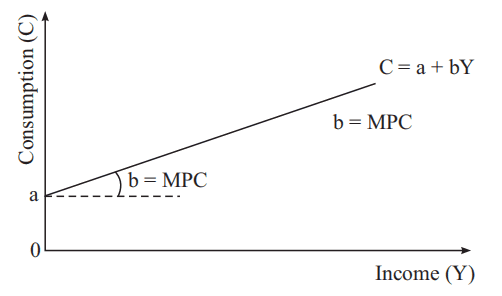
Consider a consumption function given by

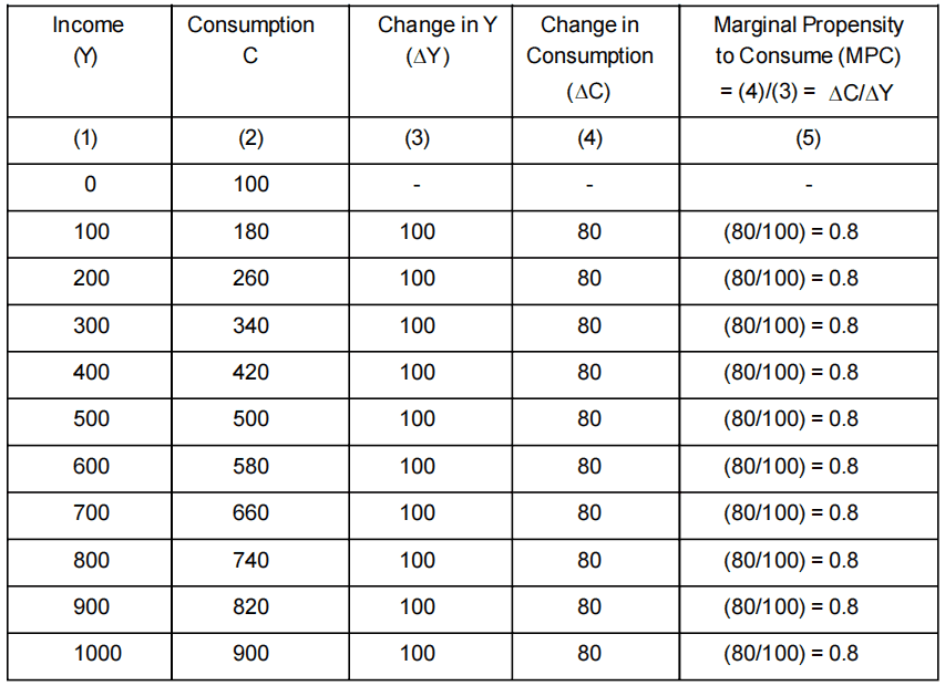
C = 100 + 0.8 Y

Since this is an equation of a straight line, the consumption function will have a constant slope.

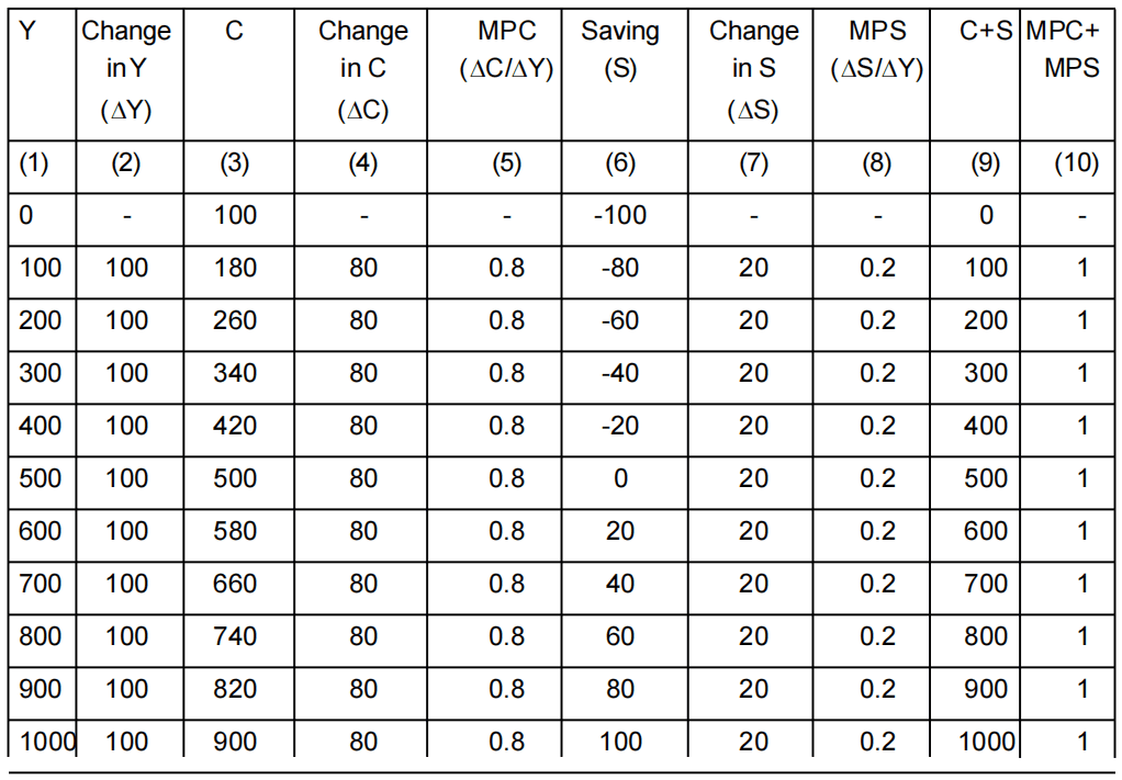
Table 1: Consumption, Income, and Marginal Propensity to Consume

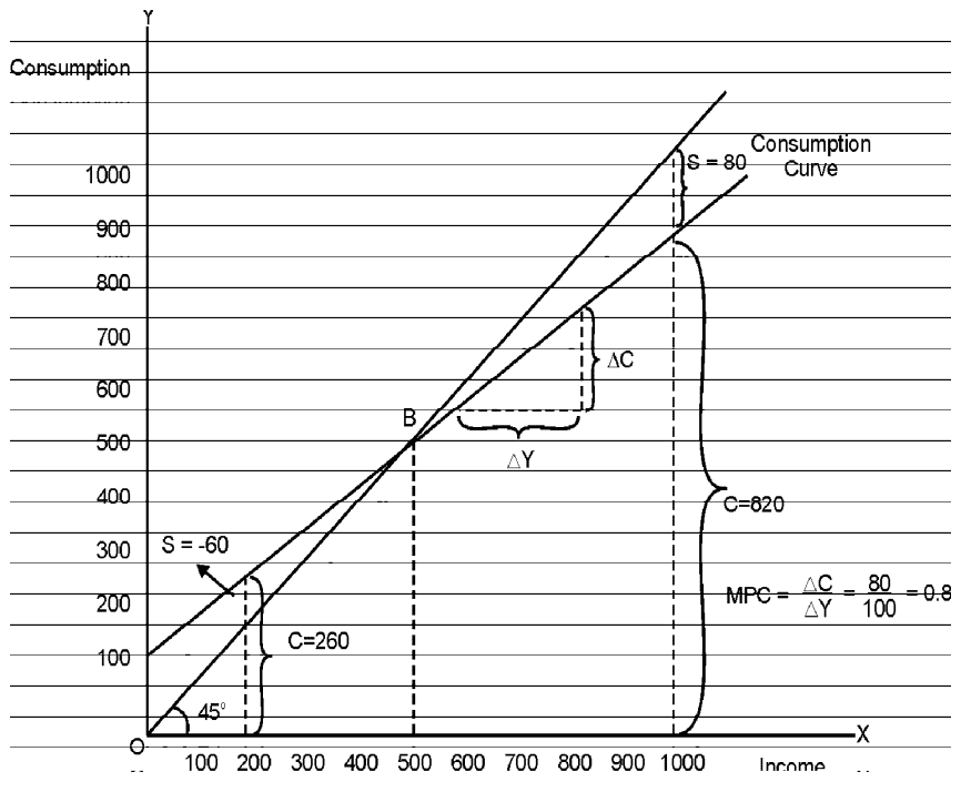
To understand the figure, it is helpful to look at the 45° line drawn from the origin. Since the vertical and horizontal axes have the same scale, the 45° line has the property that at any point on it, the distance up from the horizontal axis (which is a consumption expenditure) exactly equals the distance across from the vertical axis (which is income).

Thus, at any point on the 45° line, consumption expenditure exactly equals income. The 45° line therefore immediately tells us whether consumption spending (as per the consumption function) is equal to, greater than, or less than the level of income.

The consumption function crosses the 45° line at point B. This point is known as the breakeven point. Here households are just breaking even because the consumption is exactly equal to the income. In our example, the income and consumption at the breakeven point is ₹ 500.

At points to the left of B, the consumption function lies above the 45° line. Therefore consumption expenditure is greater than income. For example, at an income level of ₹ 200, the consumption is ₹ 260. The household must find funds to meet this consumption expenditure. The shortage in income will make them sell the assets acquired in the past, or resort to borrowing so that ₹ 60 could be raised for consumption. This act on the part of the household to liquidate their own assets or to go in for a loan is referred to as the process of dissaving. Dissaving is in order to help households to finance their consumption over and above the level of income.

At any point to the right of B, the consumption curve lies below the 45° line; therefore consumption expenditure is less than the level of income. The part of income, which is not consumed, is saved. This must be so because income is either consumed or saved. There is no other use to which it can be put. Savings can be measured in the graph as the vertical distance between the consumption function and the 45° line. For example, at an income level of ₹ 900, consumption is Rs. 820. Therefore, the amount of savings is the difference between the two, that is, ₹ 80.

Savings

We shall now look into the relationship between consumption and saving. We may obtain the savings function from this relationship.

S = Y - C

⇒ S = Y - (C̅ + bY) (Since C = C̅ + bY)

⇒ S = Y - C̅ - bY

⇒ S = -C̅ + Y - bY

⇒ S = -C̅+ (1 - b)Y

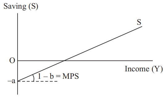
This is the savings function. The intercept term C̅ is the amount of savings done when there is a zero level of income. It is already shown that C̅ is positive. Therefore C̅ savings is negative. Thus, there is negative saving C̅ at a zero level of income. Since negative savings is nothing but dissaving, this means that at zero level of income, there is a dissaving of amount C̅.

Note that the amount of autonomous consumption is exactly equal to the amount of dissaving at zero level of income. This is because of the fact that Y = C + S (whether S is positive or negative).

The slope of the savings function is (1 - b). The slope of the savings function gives the increase in savings per unit increase in income. This is known as the Marginal Propensity to Save (MPS).

Marginal propensity to save (MPS): It is the change in savings per unit change in income. It is denoted by s and is equal to (1− b). It implies s + b = 1.

Since b is less than one it follows that (1 - b) and therefore MPS is positive. Therefore, saving is an increasing function of income. Suppose the MPC, that is, b is 0.8, then the MPS, that is (1 - b) is 0.2. This means that for every one rupee increase in income, savings increase by 0.2 rupees.

Note: MPS = 1 - b ⇒ MPS = 1 - MPC ⇒ MPC + MPS = 1

Graph of Saving function

Using the numerical example of the consumption function we had earlier given, we can derive the corresponding savings function.

C = 100 + 0.8 Y

∴ S = Y - C = Y - [100 + 0.8 Y] = Y - 100 - 0.8 Y = -100 + 0.2 Y

Consumption Savings Relationship

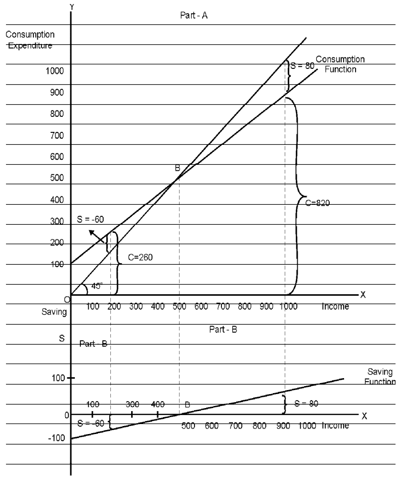
In general, to the left of point B in part A, the consumption function lies above the 45° line (consumption is more than income). Hence to the left of point B in part B, savings is negative and the savings function lies below the horizontal axis.

To the right of point B in part A, the consumption function lies below the 45° line (consumption is less than income). Hence to the right of point B in part B, savings is positive and the savings function lies above the horizontal axis.

Average Propensity to Consume and Average Propensity to Save

Average propensity to consume (APC): It is the consumption per unit of income i.e., ^C/_Y.

• It can never be zero.
• It can be greater than 1.

Average propensity to save (APS): It is the savings per unit of income i.e., ^S/_Y.

• It can be negative.
• It can be zero.

We know, Y = C + S

⇒ ^Y/_Y = ^C/_Y + ^S/_Y [dividing both sides by Y]
⇒ 1 = APC + APS

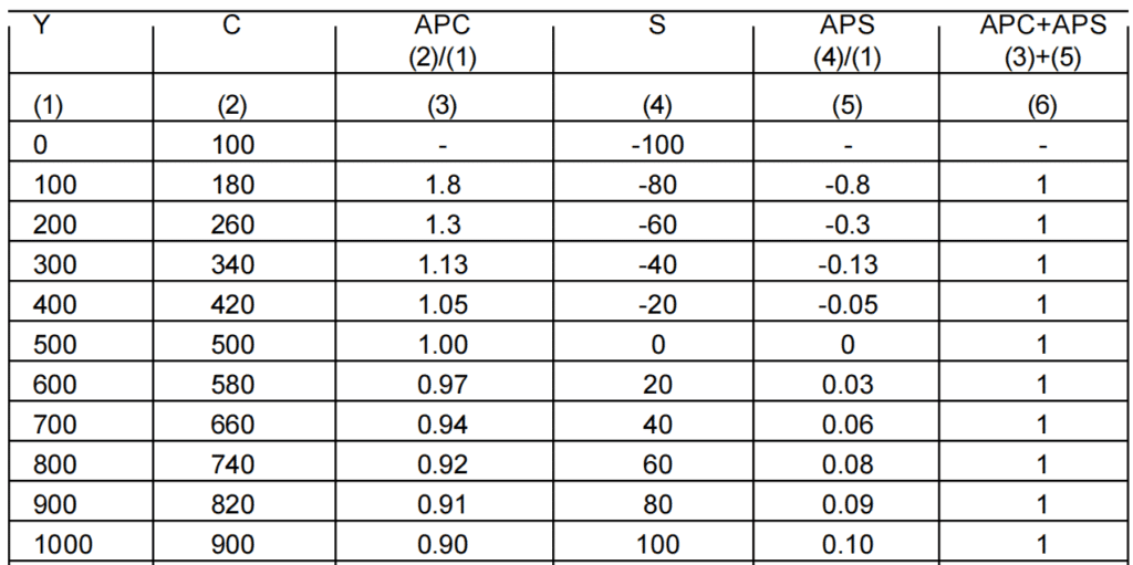
As we can see from the above table. APC is continuously declining as income increases, and APS is continuously increasing as income increases. This means that as income increases, the proportion of income saved increases and the proportion of income consumed decreases.

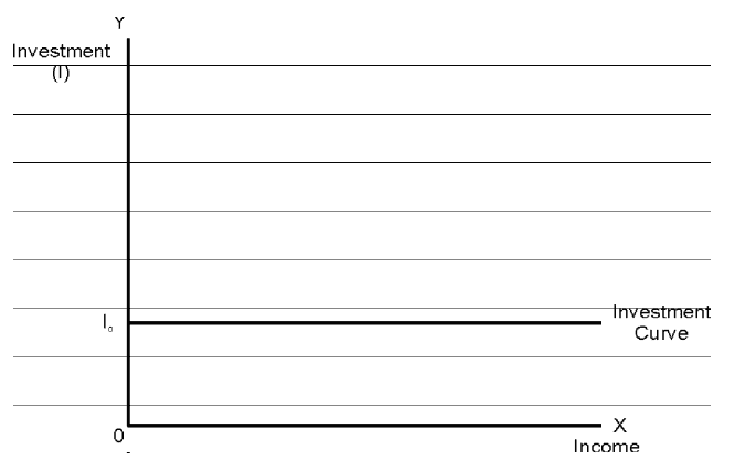
2. Demand for Private Investment

Demand for private investment refers to the planned or ex-ante investment expenditure by the firms. It includes an addition to the stock of physical capital and changes in inventory. For simplicity's sake, it is assumed in our study that the investment expenditure is autonomous. This means investment decisions are not influenced by any of its determinants, including output.

I = I₀

Aggregate Demand:

AD = C + I₀

OR

Aggregate Supply

It is the value of the total quantity of final goods and services produced in the economic territory of a country. It refers to the planned aggregate output in the economy. It can be said that the actual value of total output is the same as the economy's income. Let it be denoted as Y. It is also said that income is divided between consumption and saving.

So, Y = C + S.

Significance of the 45° line

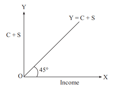
The value of output (Aggregate Supply/GDP) is the same as the level of income Y. Also Y = C + S. Geometrically on a 45-degree line through the origin Y = C + S when we measure income Y along the horizontal axis and C + S along the vertical axis. It should be noted that on a 45-degree line C + S = Y because it divides the plane into two equal parts.

Determination of Equilibrium Level of Income

We shall confine our analysis of the determination of the equilibrium level of income to an economy with only two sectors, households and firms. Hence, the only components of aggregate demand will be consumption demand and investment demand.

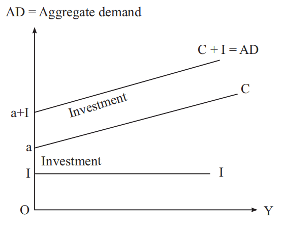
1. Consumption plus Investment (C+ I) Approach

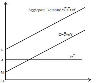
AD: The figure below shows aggregate demand plotted against income. The line CC is the consumption function, showing the desired (planned level) of consumption corresponding to each level of income. We now add desired (planned) investment (which is at fixed level I) to the consumption function. This gives the level of total desired spending or aggregate demand, represented by the C+I₀ curve.

AS: The 45° line will enable us to identify the equilibrium. At any point on the 45° line, the aggregate demand(measured vertically) equals the total level of income (measured horizontally).

Equilibrium: The economy is in equilibrium when aggregate demand, represented by the C+I₀ curve is equal to the total income.

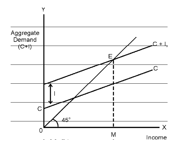
The aggregate demand or (C + I₀) curve shows the desired level of expenditure by consumers and firms corresponding to each level of output. The economy is in equilibrium at the point where the C + I₀ curve intersects the 45° line - point E in the above figure. At point E, the economy is in equilibrium because the level of desired spending on consumption and investment exactly equals the level of total income. The level of income corresponding to point E is the level of income OM. Thus, OM is the equilibrium level of income.

Algebraically,

At equilibrium, we have
Y = C + I
⇒ Y = C̅ + bY + I
⇒ Y - bY = C̅ + I
⇒ Y(1 - b) = C̅ + I
⇒ Y = ^{(C̅ + I)}/_{(1- b)}

The Adjustment Mechanism

Equilibrium occurs when planned spending equals planned income. When planned spending is not equal to planned income, then income will tend to adjust up or down until the two are equal again.

Case-I: When AS>AD

Consider the case when the economy is at a level of income greater than the equilibrium level OM. At any such greater level of income, the C + I₀ line lies below the 45° line that is planned spending is less than planned income. This means that consumers and firms together would be buying less goods than firms were producing. This would lead to an unplanned undesired increase in inventories of unsold goods (representing goods neither sold to households for consumption nor bought by firms for investment) Firms would then respond to this unplanned inventory increase by decreasing employment and hence output. This process of decrease in income will continue until the economy is back at income level OM, where again aggregate demand equals planned income and there is no further tendency to change.

Case-II: When AS<AD

Consider another case when the economy is at a level of income less than the equilibrium at level OM. At any such lower level of income, the C + I₀ line lies above the 45° line, that is, planned spending is more than planned income. This means that consumers and firms together would be buying more goods than firms were producing. This would lead to an unplanned, undesired decrease in inventories. Firms would then respond to this unplanned inventory decrease by increasing employment and hence output. This process of increase in output will continue until the economy is back at income level OM, where again aggregate demand equals planned income and there is no further tendency to change.

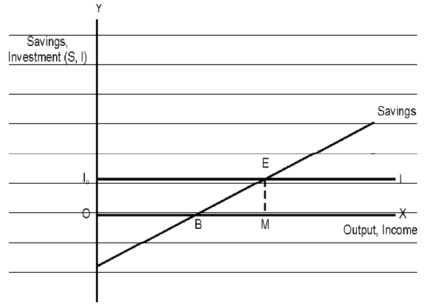
2. Saving and Investment Approach (S-I Approach)

The equilibrium level of income can be determined by using the saving and investment approach.

We know,
At equilibrium,
Y = AD
⇒ C + S = C + I
⇒ S = I

Hence whenever aggregate demand equals total output, saving also equals investment. This means that the point at which saving and investment are equal refers to the equilibrium level of income.

The Adjustment Mechanism

Case-I:

When the economy is at a level of income greater than OM. At the corresponding level of income, the savings curve lies above the investment curve, Therefore, at this level of income planned savings are more than planned investments. The effect of this will be to cause an unplanned build-up of inventories. In order to reduce the unplanned inventories to the desired level, firms will cut back production. The effect of this will be a fall in income until the economy returns to equilibrium at income level OM, where planned savings equal planned Investment.

Case-II:

When the economy is at a level of income less than OM. At the corresponding level of income, the savings curve lies below the investment curve. Therefore, at this level of income planned savings are less than planned investment. The effect of this will be to cause an unplanned, reduction in inventories. In order to increase inventories to the desired, planned level firms will increase production. The effect of this will be an increase in income till the economy returns to income level OM, where planned savings equal planned investment.

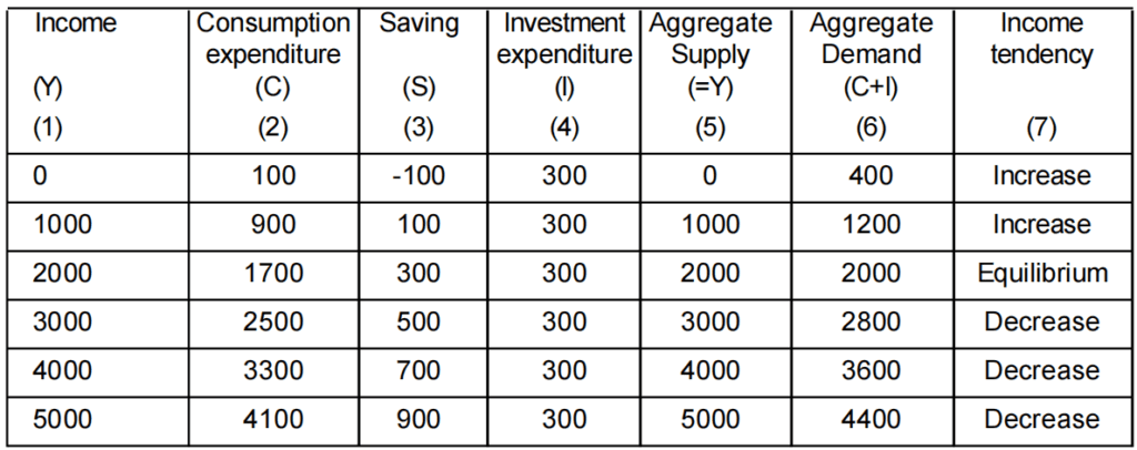
In equilibrium, Aggregate Demand equals Aggregate Supply

Let us take a numerical example to show the same. Let, C̅ = 100 and MPC = 0.8

Multiplier (Investment Multiplier)

A change in investment spending affects income.

For example, if an increase in investment of ₹ 100 crores causes an increase in income of ₹ 300 crores, then the multiplier is 3. If, instead the resulting increase in income is ₹ 400 crores, then the multiplier is 4.

i.e., K = ^ΔY/_ΔI

Derivation of Multiplier

At equilibrium, we have
Y = C + I
⇒ ΔY = ΔC + ΔI [Multiplying both sides by Δ]
⇒ ^ΔY/_ΔY = ^ΔC/_ΔY + ^ΔI/_ΔY [Dividing both sides by ΔY]
⇒ 1 = MPC + ^ΔI/_ΔY
⇒ ^ΔI/_ΔY = 1 - MPC
⇒ ^ΔY/_ΔI = ¹/_1-MPC = ¹/_MPS

• Range of Investment Multiplier = one to infinity.
• Relation:
  • if MPC rises, investment multiplier rises: positive relation,
  • if MPS rises, investment multiplier falls: inverse relation.

The Multiplier Mechanism (The Working of Multiplier)

Let the MPC be at 0.8. Suppose there is an increase in investment of Rs. 1000. which results in the construction of a new building. Then, the builder, the architect, and the laborers together will get an increase in income of Rs. 1000. Since the MPC is 0.8, they will together spend (0.8)1000 [i.e., Rs. 800] on new consumption goods. The producers of those consumption goods will thus have an increase of (0.8)1000 [i.e., Rs. 800] in their incomes. Since their MPC is also 0.8, they will in turn spend Rs. 640 [i.e., 0.8 of (0.8)1000 = (0.8)²1000]. This will cause an increase in the income of other people by Rs 640. This process will go on with each new round of spending (and therefore increase in investment) being 0.8 of the previous round.

Thus, an endless chain of secondary consumption spending is set in motion by the primary investment of Rs. 1000. However. not only is the chain of secondary consumption spending endless, but it is also ever-diminishing. Eventually, the sum of the secondary consumption expenditures will be a finite amount.

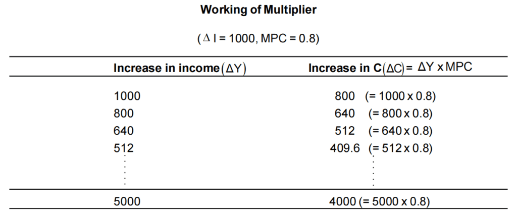
In order to find out the total increase in output of the final goods, we must add up the infinite geometric series in the last column, i.e.,

1000 + (0.8)1000 + (0.8)²1000 + .........∞

= 1000 (1 + 0.8 + 0.8² + ....... ∞)

= 1000 (¹/_1-0.8)

= 5000

Paradox of Thrift

If all the people of the economy increase the proportion of income they save (i.e. if the MPS of the economy increases) the total value of savings in the economy will not increase – it will either decline or remain unchanged. This result is known as the Paradox of Thrift – which states that as people become more thrifty they end up saving less or the same as before.

Excess Demand

We know that the equilibrium level of income is determined at the point where aggregate demand (AD) equals the level of output (Y). Let us assume that the level of output is at the maximum possible level or potential level which is achieved by full utilization of the resources of the economy. This means that the economy output will not increase beyond the potential level. We also know that an increase in AD through an increase in investment, brings about an increase in income or output due to the working of the multiplier. Now think of a situation in which the economy is already operating at its potential level of output and there is an increase in investment at that level. What will happen? Will the level of output increase further?

The answer is that the economy’s output will not increase. However, due to an increase in investment, which is a type of fixed or autonomous expenditure, the aggregate demand (AD) will increase and exceed the level of potential output. Such a situation is called excess demand in the country.

So, excess demand refers to the situation when aggregate demand exceeds the potential level of output in the economy.

The result of excess demand is inflation in the economy.

Diagrammatically excess demand is created when the AD line shifts upwards at the level of equilibrium as shown in the diagram below.

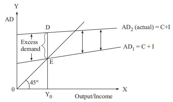
In the diagram, it is shown that the equilibrium position is at point E, where aggregate demand line AD₁ meets the 45° line. Let the economy be at equilibrium level of income. Now let aggregate demand increase from AD₁ to AD₂ due to an increase in fixed investment or consumption. As a result, a gap to the extent of DE is created which is the difference between the new and old aggregate demand. Here the income is not increasing beyond Y₀ after an increase in AD. So the gap DE is the measure of excess demand in the economy. This gap is also called the inflationary gap.

Remedy for Excess Demand

The aggregate demand may be decreased by taking recourse to fiscal policy, monetary policy, or both.

i. Fiscal Policy Measures

Excess demand can be reduced by

• decreasing the level of government expenditure
• by increasing the amount of taxes.

If the government expenditure is decreased by an amount equal to the inflationary gap, it will restore the economy to the full-employment equilibrium.

ii. Monetary Policy Measures

The following are the instruments of monetary policy.

• Bank rate: The Central Bank (RBI) can increase the Bank rate to cure inflation.
• Open market operation: Open market operation refers to buying and selling of securities by the central bank. During inflation (excess demand situation) the central bank sells government securities to commercial banks in return for money. As a result money supply in the economy falls causing prices to fall.
• Cash reserve ratio: To control excess demand, the central bank will increase the cash reserve ratio.

Deficient Demand

Deficiency in demand is exactly the opposite of excess demand situation. When the economy is at its potential level and there is a fall in aggregate demand due to a fall in autonomous consumption or investment, then it is called a deficient demand. In this situation, the output level seems to be in surplus in the market and people do not demand it thus putting pressure on the price level to fall in order to balance the demand and supply forces. This creates deflationary pressure in the economy where deflation implies a fall in the prices of goods and services.

Diagrammatically, deficiency in demand is shown by the fall in the AD line at the level of potential output as shown below in the diagram.

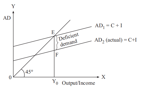
In the diagram, equilibrium income is determined at point E where the original aggregate demand, AD1 cuts the 45° line. The corresponding income at Y₀ is the potential level. Now at this level, AD₁ falls to AD₂ creating a gap EF without any fall in output. EF is the measure of deficient demand. This gap is also called the deflationary gap.

Remedy for Deficient Demand

The aggregate demand may be increased by taking recourse to fiscal policy, monetary policy, or both.

i. Fiscal Policy Measures

Deficient demand can be increased by

• increasing the level of government expenditure
• by decreasing the amount of taxes.

If the government expenditure is increased by an amount equal to the deflationary gap, it will restore the economy to the full-employment equilibrium.

ii. Monetary Policy Measures

The following are the instruments of monetary policy.

• Bank rate: The Central Bank (RBI) can decrease the Bank rate to cure deflation.
• Open market operation: Open market operation refers to buying and selling of securities by the central bank. During inflation (excess demand situation) the central bank buys government securities from commercial banks. As a result money supply in the economy increases causing prices to rise.
• Cash reserve ratio: To control deficient demand, the central bank will decrease the cash reserve ratio.

Involuntary unemployment: Involuntary unemployment occurs when those who are able and willing to work at the going wage rate do not get work. It is distinguished from Voluntary unemployment which refers to the part of the population which is able to work but voluntarily prefers not to work.

Full Employment: When the entire labor force of the country is in employment, it is called full employment. The labor force comprises people who are able to work and willing to work.

Also, See: Determination of Income and Employment Class 12 Important Questions Answers Money and Banking Class 12 Notes

Also Read: Class 12 Important Questions Class 12 Notes

Hope you liked this Notes on Class 12 Economics Determination of Income and Employment. Please share this with your friends and do comment if you have any doubts/suggestions to share.